
Google Sheets Examples
Downloading and importing data
To download your data, you’re going to start in the Wish List app, and click on the “Reports” section:
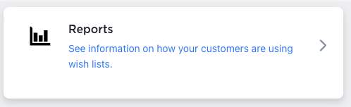
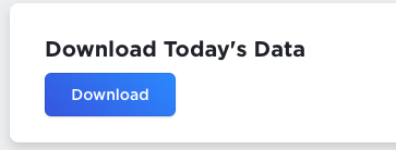
From here, you’ll see a “Download” button where you can get your current data. This data is generated every day at around midnight, UTC time. It will give you the last two months worth of data, where any of your customers who are signed in will have their wish list information appear.
Once you have the data downloaded, you should have a CSV file with today’s date as the file name. In Google Sheets, you’re going to want to import the data into a spreadsheet – this can be a new spreadsheet or you can choose to organize your imports as you see fit.
To import the data, you’ll need to go yo the “file” menu, and select the “import” option.
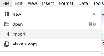
From here, you’ll be given some options on what to do. Since I’m importing to a new spreadsheet, the default options are acceptable to me.
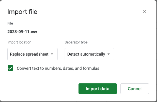
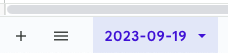
When the import is done, you’ll see that the sheet name is the same as the name of the file that we imported. If you were doing something like importing all of these files to one spreadsheet each day, you could set the “Import location” option to something like “Insert new sheet(s)” and you would see different sheets at the bottom with different dates.
Filtering your data
Chances are you won’t be working with all of this data at once, so we’ll need to create filters to get you just the data you’re looking for.
To create filters, select the header row from your sheet by clicking on the “1” next to the “Customer Email” cell, to select the entire row.

Next, click on the “Data” menu at the top of the window, and click on the “Create a filter” option.
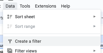
You should see a change in your data, where there should be small filter icons next to each title, and each title should be in a bold font now.

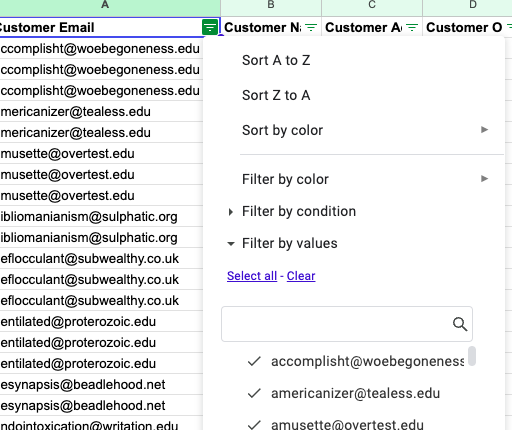
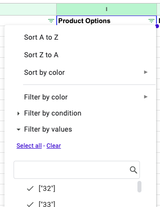
When you select one of these options, you should be able to see all of the different values for what you’ve selected. In this exmaple below, I’ve selected the filter for “Customer Email” by clicking on the filter icon, and I can see all of my customer emails in this data, at the bottom of the options. From here, I can manually select or deselect the emails I’m looking for, or I could quickly look through the data for specific email addresses by typing in the search bar, above those email addresses.
For most of the options, this is probably fine, but if I have multiple available product options, they’re going to appear in a list where selecting by what the text says probably isn’t quite what I’m looking for.
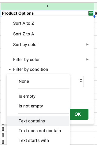
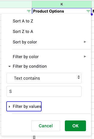
In this case, I’m probably looking for a different filter type. The one I’d probably want to use is the “text contains” filter, which can be selected from the “Filter by condition” section.
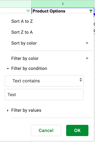
With that filter selected, I can now do a search for exactly what I’m looking for. In the example below, I’m doing a search for people who have used the “Test” option on one of their products, but in real life you’d probably be searching for something more like a size or color option. This filter should find those without problems in this same way.
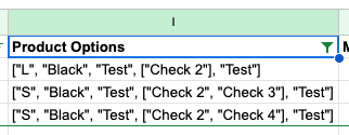
With that filter on, I’m now only getting a few rows in my data.
You can mix and match filters to find exactly the customers you’re looking for – you could do something like turn on filters for a pair of jeans, size 32, for customers with 0 orders, or a product from the “tshirts” product category, with the “red” product option.
There are many filters available that you can test out. You could try changing the dates to use date ranges, or prices, or any of the number values to match other logical requirements as well.
Creating a mailing list
Once you’ve found a set of people that are of interest to you, you can then take this data and turn it into a mailing list of software like Mailchimp, or Klaviyo.
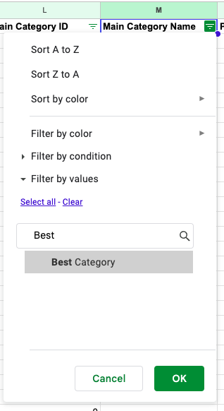
In this example, we have a sheet with 136 wish list products added that we’re sorting through. We’re going to look for people who have items from the “Best Category” or “Default Category” categories of products, who are looking at products that have the small (“S”) product option.
First we filter to the correct categories:
Then the correct product option:
And we’re left with just a few rows from the sheet:
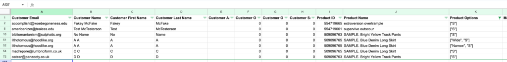
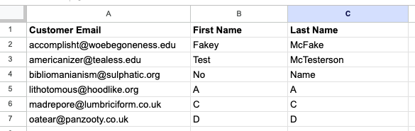
There are a couple of things left to do with this: we need to format the titles to match what our mail platform expects, and we need to remove duplicates, in case the platform we’re using doesn’t do that for us. In this case, you’ll see that “A A” with the email address “lithotomous@hoodlike.org” appears twice, because this person wanted both the narrow and wide versions of the “SAMPLE. Blue Denim Long Skirt” product. By default, Mailchimp only needs an email address, a first name and a last name, so let’s clean this up.
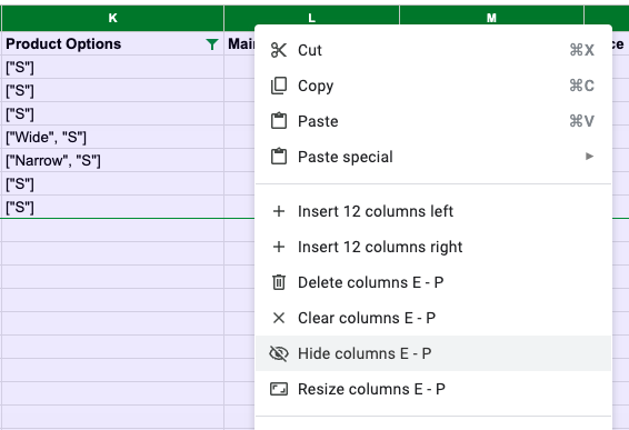
First, let’s hide the columns that we don’t need. We can do this by selecting the “B” column by right clicking on the “B” at the top of our data, and clicking the “Hide” option:
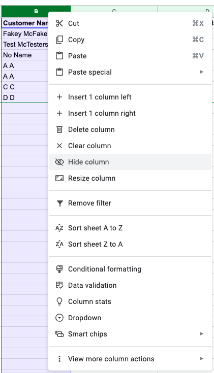
We can do the same for the rest of the columns we don’t need, by selecting columns E-P and hiding them through the same right-click menu:
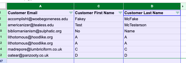
After this, we only have a few things left to clean up:
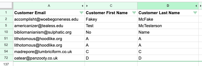
The easiest way to clean this up would probably be to copy and paste this data into a new sheet. To do this, hold the control key (command key on a mac) and click on the column names A, C and D:
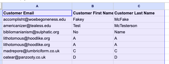
Copy the selected columns, and paste them into a new sheet:
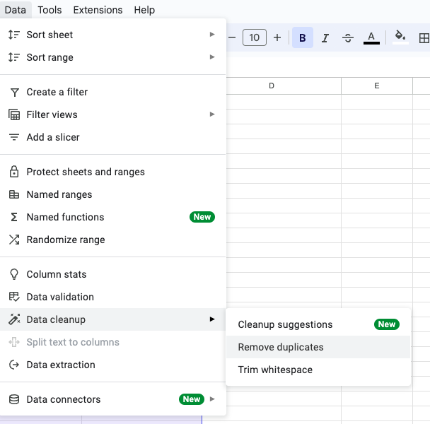
We can the remove the duplicate row from “A A” by using Google Docs’ “remove duplicates” function, by going to Data, Data cleanup, and selecting “Remove duplicates”:
Select “Data has header row” in the options, and click the “Remove duplicates” button, and we should get a confirmation message letting us know how many rows were removed. Lastly, Mailchimp wants the rows with our names in them to be called “First Name” and “Last Name”, so we can rename those columns, and we’ll be left with clean data for our upload to Mailchimp.
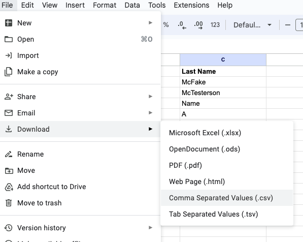
The last thing to do is to export a CSV of this data by going to File, Download and selecting Comma Separated Values in the menu.
Working with support
There are many possibilities for what you might want to do with this data. Different mailing list software might want different columns, and most of that software can take more columns than this example provided.
If you’r ever running into problems or could use some help with getting things working for you, please reach out to support at support@athousandapps.com and we’ll do what we can to help out.